The Inefficient Terrain Generator (THINTEGEN)
last updated April 2019
My most recent evening project, a raster terrain generator! It´s
quite slow compared to similar products and generally less flexible, so
I decided to name it ‘The Inefficient Terrain Generator’, or
THINTEGEN for short. It is available as an R package and
the latest version can be downloaded from my github page in
.tar.gz form.
v.0.2.0
April 5th, 2019
There are some quite important additions to this new version of
thintegen! Three new functions!
1. cubint
With the thintegen project I would really like to limit
my dependence on other R packages to the bare minimum. It makes things
more challenging, and forces me to go a bit beyond just downloading what
I need. So after experimenting with LOESS interpolation in
loint, I tried to implement something similar from scratch.
My choice fell on cubic interpolation right after stumbling upon the
formula I needed (found here after watching
a much helpful episode of
Computerphile). As much as I am fascinated by it, math is not
exactly my thing, so it took a bit trying to understand how to make it
work. Eventually everything fell into place though, and the function
cubint was born.
It works quite well if you ask me. Or, at least, it does what I need it to do. Here is a comparison with LOESS:
library(thintegen)

#testing function cubint().
#It interpolates smoothly between given points preserving their original values.

x <- c(1,5,10,20)
y <- c(0.5,7,5,10)

samp <- 0.5

#cubic
v <- cubint(x,y,samp)


#LOESS
lo <- loess(y ~ x, span=0.5)
pred <- predict(lo, seq(min(x),max(x),samp))


plot(x= seq(min(x), max(x),samp), y= v, type="o", cex=0.5, ylab="y", xlab="x",xlim=c(min(x),max(x)), ylim=c(min(y),max(y)), col="green")

lines(x= seq(min(x),max(x),samp), y= pred, type="l", cex=0.5, col="purple")

points(x,y,col="black", pch=19)

legend("topleft",
        legend = c("cubint()", "LOESS"),
        col = c("green","purple"),
        lty=1:1,
        pch=c(1,NA),
        bty = "n")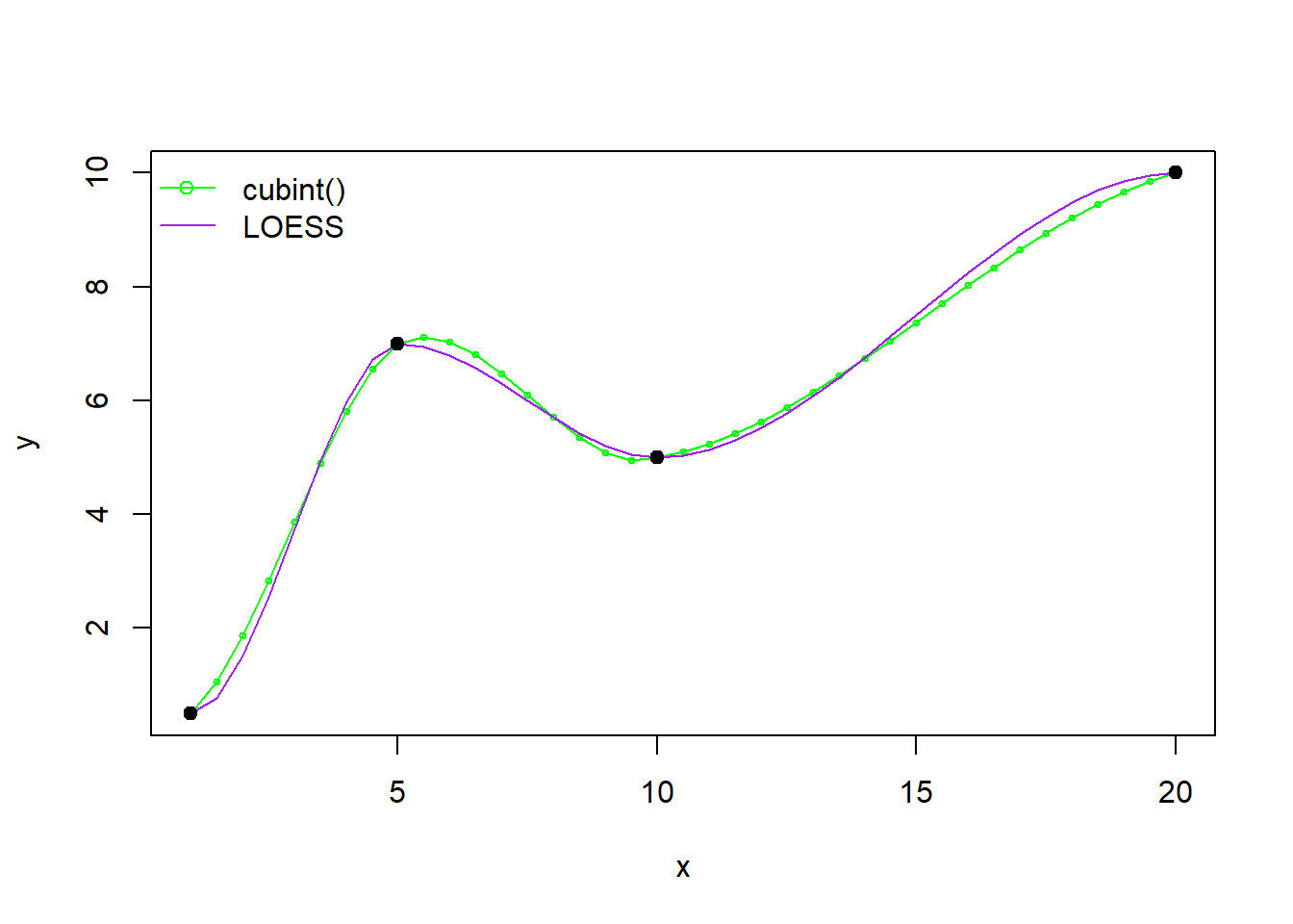
Sure, cubint does not have any adjustable smoothing
parameter, which makes it somewhat not very flexible. But it complains
much less than loess when the parameters are not optimal or
are insufficiently tuned (because, well, there is nothing to tune in
cubint), and that´s why I like it.
2. bicubint
After producing my very own interpolation function, it was time to
put it to test. I took the core of loint and pretty much
replaced the loess function with cubint. The
algorithm still operates row-wise and column-wise at increasing
frequencies, resulting in a sort of primitive bicubic interpolation and
in, well… the bicubint function. Drawing from Perlin noise
and from an already mentioned great video from Sebastian
Lague, I introduced octaves, lacunarity and persistence to modulate the
frequency and amplitude of the interpolation. The result was actually
quite surprising. Compared to loint, bicubint
is faster and produces more organic and Perlin-like results. Also, I
made bicubint more adjustable, with the options to pick
different x and y dimensions, as well as horizontal and vertical cell
counts. I´m planning to bring all these improvements to
loint too as soon as I have time.
Here is a raster map produced with bicubint:
library(thintegen)

r <- bicubint(x_dims=c(-150,200),y_dims=c(-100,250), octaves=c(1:3),lacunarity=10, persistence=0.3)

library(raster)
crs(r) <- CRS('+init=EPSG:6933')
slope <- terrain(r, opt='slope')
aspect <- terrain(r, opt='aspect')
hill <- hillShade(slope, aspect, 40, 270)

par(mfrow=c(1,2), oma=c(0,1,0,1), mar=c(6,1,6,1))

plot(hill, col=grey(0:100/100), legend=FALSE, main="hillshade")

plot(r ,col=terrain.colors(255), main="elevation")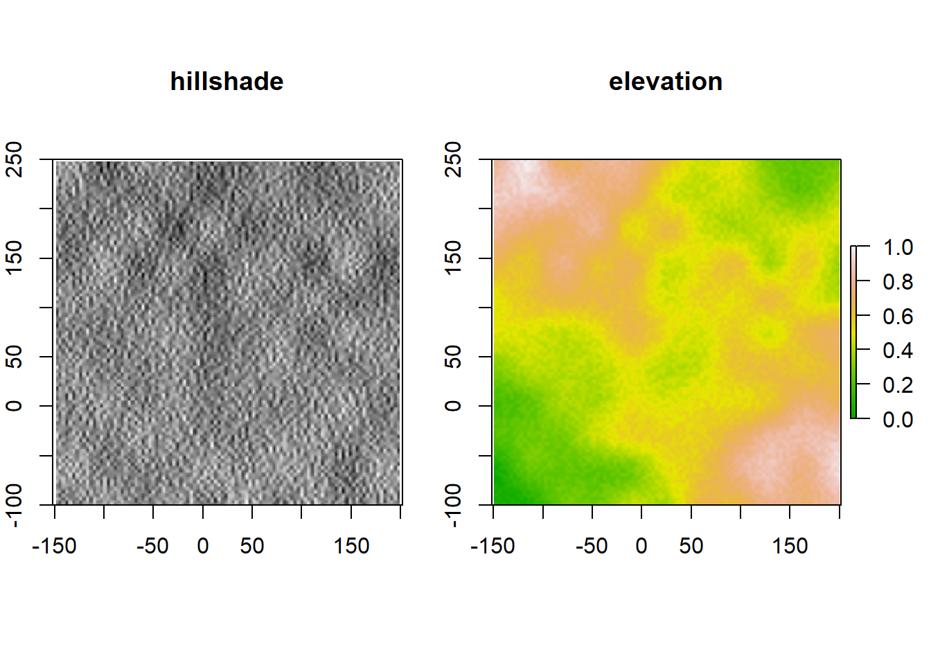
3. smoothcrawler
Both loint and bicubint are quite rough and
might produce some nasty looking interpolation artifacts or jagged
surfaces. Sometimes it’s possible to get rid of those by adjusting some
parameters, and sometimes a dedicated function might be needed to solve
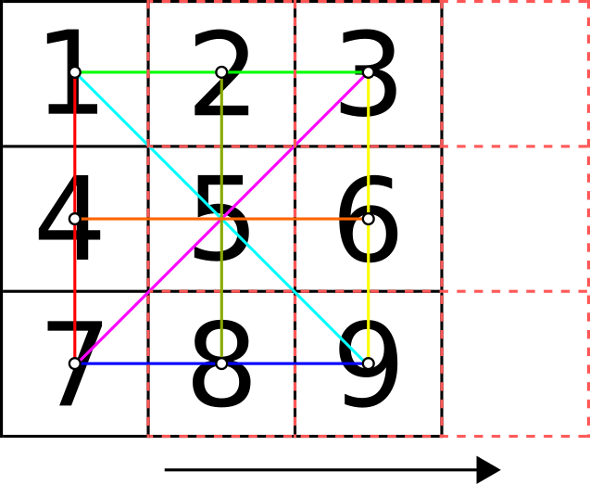
the issue. Enter smoothcrawler. This function takes a 3x3
matrix and alters the content of every cell comprised between each pair
of corner values. For instance, in the example below it would take the
values of cells 1 and 3, and average them to get the value of two. The
process is then repeated for cell 4 using the values of 1 and 7, and so
on. After getting the values of 2,5,6 and 8, the content of cell 5 is
calculated via every possible combination of opposite surrounding cells.
All the newly produced values for each cell are then averaged together
with the original ones in their respective positions. If
smoothcrawler is applied to a matrix bigger than 3x3, it
moves by one cell to the right after every cycle and repeats the
averaging procedure. After a full row is completed, it moves to the far
left of the matrix, shifts down by one cell, executes the averaging and
so on, eventually crawling across the whole matrix.
It’s quite aggressive, and in the future I might add some options to tone it down a bit. But, for the moment, it works as intended!
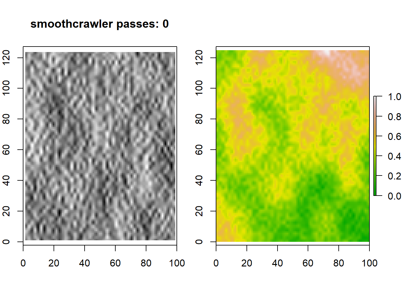
Here is a first example:
library(thintegen)
library(raster)


#producing a raster file with bicubint

r <- bicubint(x_dims=c(0,100),y_dims=c(0,125), octaves=c(1:3),lacunarity=7, persistence=0.5)


#apply smoothcrawler 0, 1 and two times to the same map

for (i in c(0,1,2)) {

r1 <- smoothcrawler(r, passes=i)


crs(r1) <- CRS('+init=EPSG:6933')
slope <- terrain(r1, opt='slope')
aspect <- terrain(r1, opt='aspect')
hill <- hillShade(slope, aspect, 40, 270)

par(mfrow=c(1,2), oma=c(0,1,0,1), mar=c(4,1,4,1))
plot(hill, col=grey(0:100/100), legend=FALSE, main=paste("smoothcrawler passes: ",i, sep=""))
plot(r1 ,col=terrain.colors(255), main=NA)

}
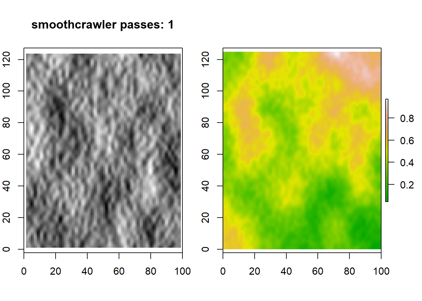
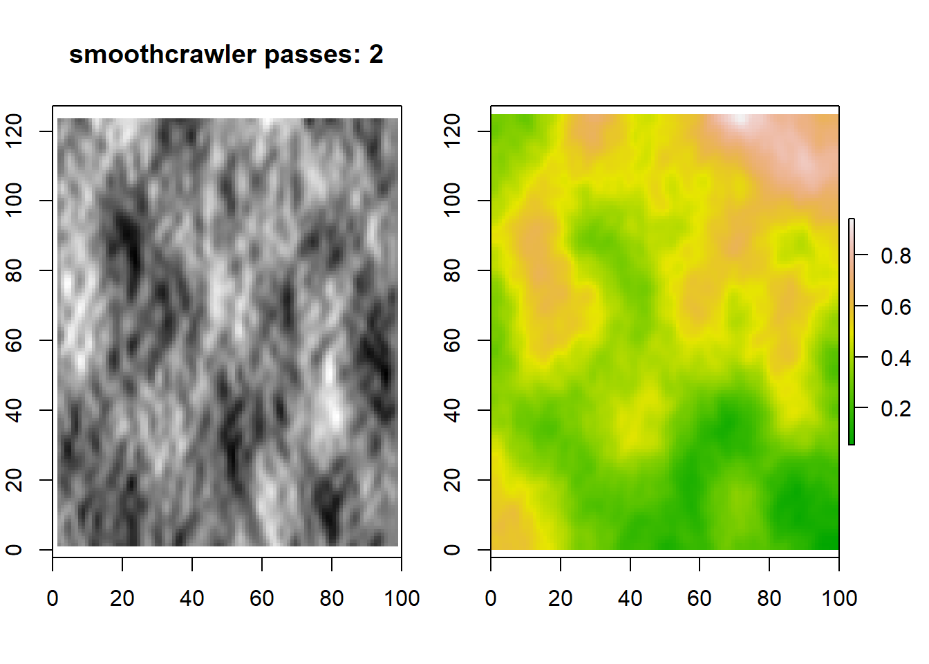
A similar smoothing can be achieved by playing with the parameters in
the bicubint function, especially persistence. Still, the
smoothcrawler has also the ability to discriminate between
z values, smoothing only across selected intervals. Like in this
example:
#generate a random terrain with the bicubint() function

r <- bicubint(x_dims=c(0,750),y_dims=c(0,500),
              min_z=0,max_z=10,octaves=c(1:3),
              lacunarity=10,persistence=0.5)

#smooth the whole raster five times

r <- smoothcrawler(r, c(0:10), passes=5)

#smooth ten additional times z values >= 4 and <= 6.
#smooth five additional times z values >= 0 and <= 3.5.
#big maps are less affected by individual passes than smaller ones, requiring more iterations to achieve some visible smoothing.

r <- smoothcrawler(r, c(4:6), passes=10)
r <- smoothcrawler(r, c(0:3.5), passes=5)

#plot the output

library(raster)

crs(r) <- CRS('+init=EPSG:6933')
slope <- terrain(r, opt='slope')
aspect <- terrain(r, opt='aspect')

hill <- hillShade(slope, aspect, angle = 45, direction = 45, normalize = TRUE)
plot(hill, col = grey(0:100/100), legend = FALSE)
plot(r, col = topo.colors(255, alpha = 0.45), add = TRUE)
plot(r, col = grey(0:100/100, alpha = 0.45), add = TRUE)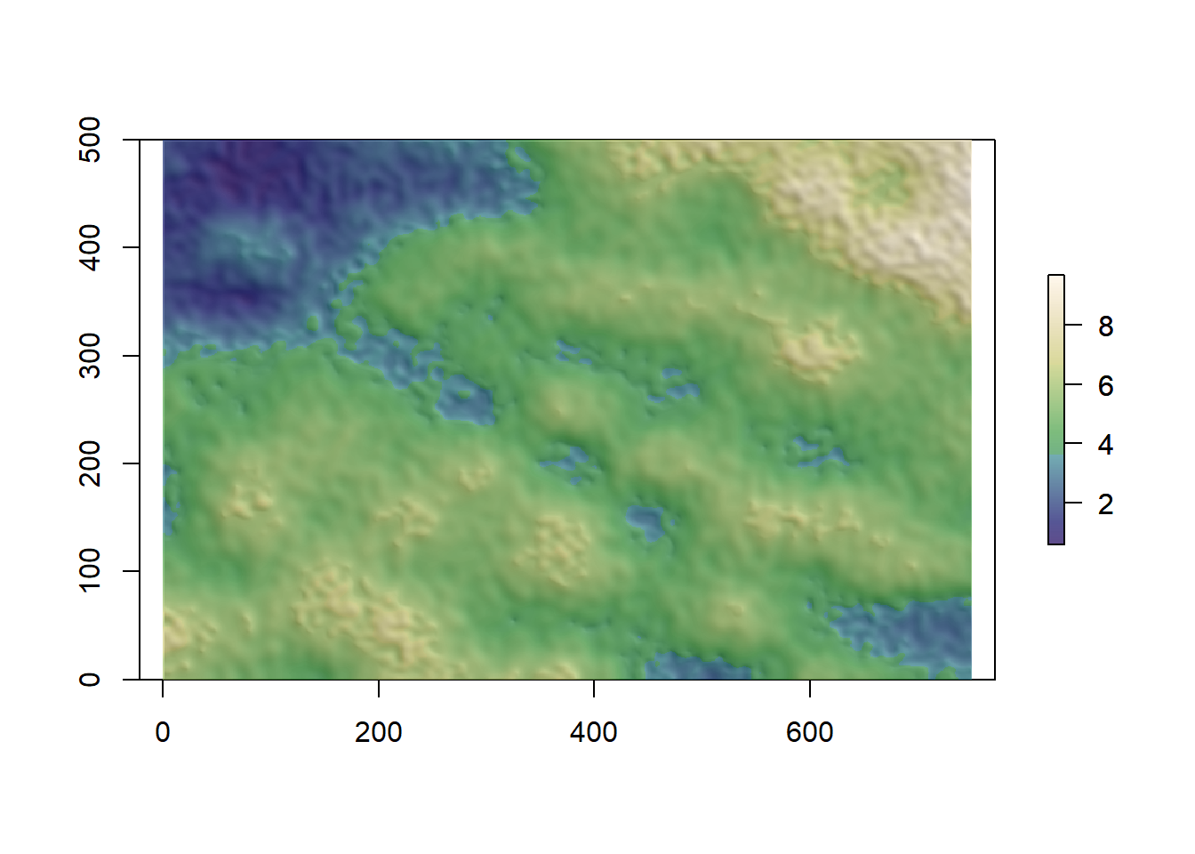
I might be getting closer to make some decent-looking artificial maps.
v.0.1.0
March 24th, 2019
Some weeks ago, I stumbled upon a great series of videos produced by Sebastian Lague on Procedural Landmass Generation. Now, at this stage I know pretty much nothing about Unity and even less about C# scripting, but the idea of producing a terrain generator still intrigued me quite a lot, so I had to give it a try with the tools at hand (that is: R).
I should also add that right now I have no idea how to implement Perlin noise in R. If you are specifically looking for that (or for something in general more capable than this project of mine), you should most definitely take a look at this Stackoverflow post, or install the ambient package.
Currently there is only one function available in thintegen,
loint. What it does is put a bunch of random points on a
grid and then LOESS-interpolate them row-wise, column-wise and
diagonal-wise until all cells are filled. Why I picked LOESS
interpolation? No reasons other than it was the first one I thought
about while writing the code!
Here are a few examples up to 500X500 grid cells produced with standard settings:
library(thintegen)

for (i in c(100,250,500)) {

r <- loint(size=i)

library(raster)
crs(r) <- CRS('+init=EPSG:6933')
slope <- terrain(r, opt='slope')
aspect <- terrain(r, opt='aspect')
hill <- hillShade(slope, aspect, 40, 270)


#eval(parse(text=noquote(paste("jpeg('./r_",i,".jpg', width = 500, height = 360, units = 'px')", sep="")))) #Jpeg export. I´ll just leave it here.
par(mfrow=c(1,2), oma=c(0,1,0,1), mar=c(6,1,6,1))
plot(hill, col=grey(0:100/100), legend=FALSE, main=paste("hillshade ",i,"x",i,sep=""), xlim = c(0,i), ylim=c(0,i))
plot(r, col=terrain.colors(255),legend=TRUE, main=paste("elevation ",i,"x",i,sep=""), xlim = c(0,i), ylim=c(0,i))
#dev.off()

}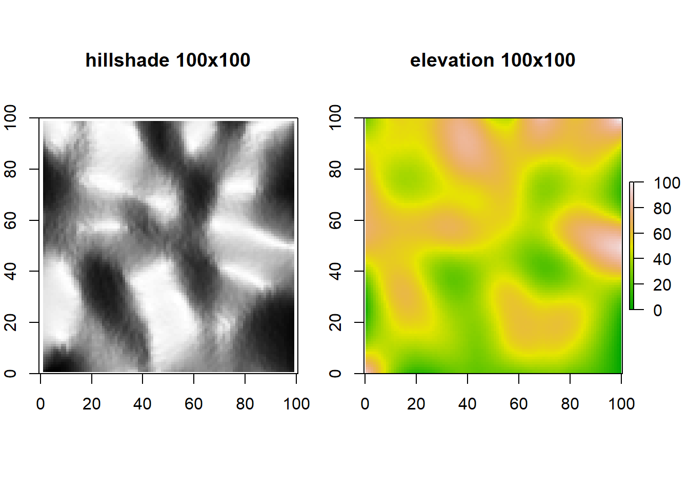

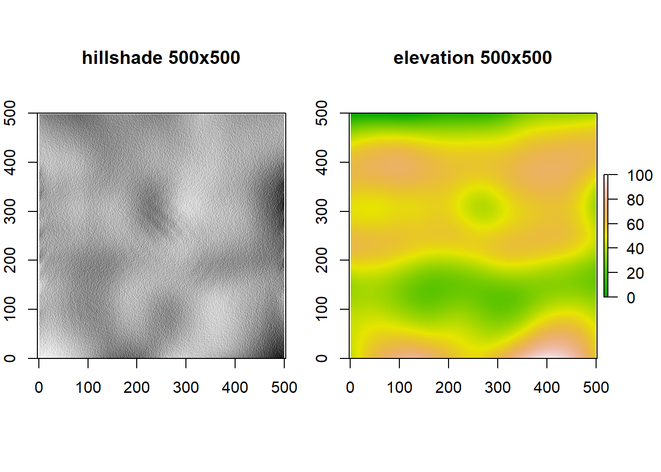
The script generates quite a bit of warning messages (all coming from the LOESS smooth parameters, which can be adjusted), it loses dynamicity at high grid cell counts, can still produce some awful interpolation artifacts and is slow as hell. But hey, it surely works as intended!
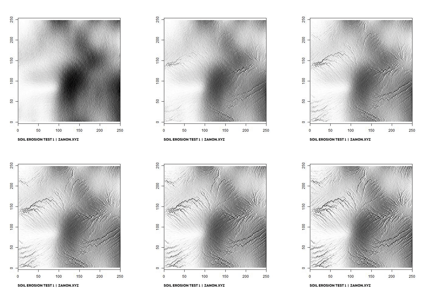
One last thing! This whole side project was born because of another YouTube video by Sebastian Lague on erosion modeling. I found the idea of simulating hydraulic erosion absolutely interesting and the results shown in the video are pretty amazing. So naturally I wanted to replicate something like that myself just to see what kind of challenges it would entail. You can see a first version of this R-based model below. the animation shows the gradual impact of 10.000 flow paths on a 250x250 elevation raster (and now you understand why I decided to build a terrain generator!). It´s still very rough but I plan to add it to THINTEGEN as soon as I’m happy with it!
